Build Qwen3 from Scratch

In this post, I will build Qwen3 model using PyTorch from scratch. I will explain the details of each component, and implement them step by step.

The reason I choose Qwen3 is that it has a 0.6B model, which is small enough to run on a single GPU, and it has most of the features that I need for better understanding of LLMs.

Model Architecture

Here is the high-level architecture of Qwen3:

I draw this diagram using Excalidraw and use Sebastian Raschka’s Qwen3 architecture diagram as a reference.

Implementation

The follwoing sections will explain the details of each component, and implement them in PyTorch. I will build the model using a top-down aapproach, starting from the overall architecture and then going down to the individual components.

Configuration

First, we define the configuration of Qwen3. This is a dataclass that contains all the hyperparameters of the model.

from dataclasses import dataclass
import torch

@dataclass()
class Qwen3Config:
    vocab_size=151936
    hidden_size=1024
    intermediate_size=3072
    num_hidden_layers=28
    num_attention_heads=16
    num_key_value_heads=8
    head_dim=128
    hidden_act="silu"
    max_position_embeddings=40_960
    rms_norm_eps=1e-6
    tie_word_embeddings=False
    rope_theta=10000.0
    dtyp=torch.bfloat16

We don’t need understand all the hyperparameters here, but I will explain them in detail later.

Model

The overall model is implemented in the Qwen3ForCausalLM class, which contains two main components: the Qwen3Model, which is the main transformer model, and the lm_head, which is a linear layer that maps the hidden states to the vocabulary size for language modeling.

class Qwen3ForCausalLM(nn.Module):
    def __init__(self, config: Qwen3Config):
        super().__init__()
        
        self.model = Qwen3Model(config)
        
        self.lm_head = nn.Linear(config.hidden_size, config.vocab_size, bias=False)

    def forward(self, input_ids: torch.Tensor) -> torch.Tensor:

        # [batch, seq_len, hidden_size]
        x = self.model(input_ids)

        # [batch, seq_len, vocab_size]
        x = self.lm_head(x)

        return x

The Qwen3Model class implements the main transformer model, which consists of an embedding layer, multiple transformer blocks, and a normalization layer.

import torch
import torch.nn as nn
import torch.nn.functional as F

class Qwen3Model(nn.Module):
    def __init__(self, config: Qwen3Config):
        super().__init__()
        self.config = config
        
        self.embed_tokens = nn.Embedding(config.vocab_size, config.hidden_size)
        
        self.layers = nn.ModuleList([
            TransformerBlock(config) for _ in range(config.num_hidden_layers)
        ])
        
        self.norm = nn.RMSNorm(config.hidden_size, eps=config.rms_norm_eps)
        
    def forward(self, input_ids: torch.Tensor) -> torch.Tensor:
        # input_ids shape: [batch, seq_len]
        
        # [batch, input_ids, hidden_size]
        x = self.embed_tokens(input_ids)

        for layer in self.layers:
            x = layer(x)

        # shape not change
        x = self.norm(x)

        # [batch, input_ids, hidden_size]
        return x

The model input is a batch of tokens with shape [batch, seq_len], after enbedding, the token embedding is passed through a series of transformer blocks, and finally passed through norm layer, and finally passed through a linear layer to get the logits. The logits has shape [batch, seq_len, vocab_size], and we can get the output tokens by taking the argmax of the logits.

model = Qwen3ForCausalLM(config)
input_ids = torch.randint(0, config.vocab_size, (2, 10)) # batch = 2, seqlen = 10
# [batch, seq_len, vocab_size]
logits = model(input_ids)
# [batch, seq_len]
next_tokens = torch.argmax(logits, dim=-1)

In the code above, I use random input tokens for testing, in real use case, the input tokens are generated by a tokenizer from text.

In the Qwen3 model implementation, I follow the official model architecture closely. In fact, I use the official model documentation and the model weights as reference, and I use the same class hierarchy and the same member names as the official pretrained model, that makes it easier to load the pretrained weights, I will explain this later.

RMSNorm

I use torch’s built-in RMSNorm implementation, which is available in PyTorch 2.0 and later. RMSNorm is a normalization technique that normalizes the input by its root mean square (RMS) value. Here is the formula of RMSNorm:

where $N$ is the number of elements in $x$, $\epsilon$ is a small constant to prevent division by zero, and $\gamma$ is a learnable scaling parameter.

We can implement RMSNorm as follows:

import torch
from torch import nn


class RMSNorm(nn.Module):

    def __init__(self, dim: int, eps: float = 1e-6) -> None:
        super().__init__()
        self.eps = eps
        self.gamma = nn.Parameter(torch.ones(dim))

    def forward(self, x: torch.Tensor) -> torch.Tensor:
        var = x.pow(2).mean(dim=-1, keepdim=True)
        rms = torch.sqrt(var + self.eps)
        x = x / (rms + self.eps)
        return x * self.gamma

After RMS normalization, the input will have a mean of 0 and a standard deviation of 1, which helps to stabilize the training process.

Why it has a mean of 0? Because the input is divided by its RMS value, which is always positive, so the output will have the same sign as the input. If the input has a mean of 0, then the output will also have a mean of 0.

Transformer Block

The Transformer Block is the core component of Qwen3. It consists of two parts: the self-attention layer and the MLP layer.

Here is the implementation of the Transformer Block.

class TransformerBlock(nn.Module):
    def __init__(self, config: Qwen3Config):
        super().__init__()

        self.input_layernorm = nn.RMSNorm(config.hidden_size, eps=config.rms_norm_eps)

        self.self_attn = Qwen3Attention(config)

        self.post_attention_layernorm = nn.RMSNorm(config.hidden_size, eps=config.rms_norm_eps)

        self.mlp = Qwen3MLP(config)

    def forward(self, x):
        shortcut = x
        x = self.input_layernorm(x)
        x = self.self_attn(x)
        x = x + shortcut

        shortcut = x
        x = self.post_attention_layernorm(x)
        x = self.mlp(x)
        x = x + shortcut

        return x        

Attention

The attention mechanism in Qwen3 is called Grouped-Query Attention (GQA). In Multi-Head Attention (MHA), the number of heads of QKV are the same, but in GQA, the number of heads of Q multi times the number of heads of KV.

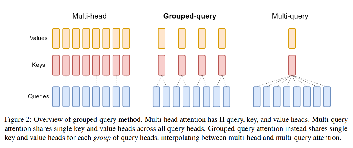
In MHA, the input is projected into three different spaces: Q, K, and V, and they have same dimension. The QKV are splited into multiple parts, each part is called a head.

Here is what MHA looks like:

In the diagram above, the input goes through multiple linear layers. But in real implementation, the input is passed through a single linear layer, and the output is split into multiple parts. But in theory, both ways have the same effect.

In GQA, the number of heads of Q is different from the number of heads of KV. Mutiple queries share the same key and value. It looks like this:

In the diagram above, we can see that keys and values are shared among multiple queries.

Here is the implementation of Grouped-Query Attention (GQA):

class GroupedQueryAttention(nn.Module):
    def __init__(self, config: Qwen3Config):
        super().__init__()

        self.config = config

        self.q_proj = nn.Linear(config.hidden_size, config.num_attention_heads * config.head_dim, bias=config.attention_bias)
        self.k_proj = nn.Linear(config.hidden_size, config.num_key_value_heads * config.head_dim, bias=config.attention_bias)
        self.v_proj = nn.Linear(config.hidden_size, config.num_key_value_heads * config.head_dim, bias=config.attention_bias)

        self.o_proj = nn.Linear(config.num_attention_heads * config.head_dim, config.hidden_size, bias=config.attention_bias)

        self.scale = self.config.head_dim**-0.5


    def forward(self, x):
        batch, seqlen, _ = x.shape
        q = self.q_proj(x)
        k = self.k_proj(x)
        v = self.v_proj(x)

        q = q.view(batch, seqlen, self.config.num_attention_heads, self.config.head_dim)
        k = k.view(batch, seqlen, self.config.num_key_value_heads, self.config.head_dim)
        v = v.view(batch, seqlen, self.config.num_key_value_heads, self.config.head_dim)

        # [batch, qhead, seqlen, head_dim]
        q = q.transpose(1, 2)
        # [batch, kvhead, seqlen, head_dim]
        k = k.transpose(1, 2)
        v = v.transpose(1, 2)


        group_size = self.config.num_attention_heads // self.config.num_key_value_heads
        
        # [batch, kv_head * group_size, seqlen, head_dim]
        k = k.repeat_interleave(group_size, dim=1)
        v = v.repeat_interleave(group_size, dim=1)


        scores = q @ k.transpose(-2, -1)
        mask = torch.triu(torch.ones(seqlen, seqlen, device=x.device, dtype=torch.bool), diagonal=1)
        scores = scores.masked_fill(mask, -torch.inf)
        scores = scores * self.scale
        weights = F.softmax(scores, dim=-1)

        # [batch, q_head, seqlen, head_dim]
        o = weights @ v

        # [batch, seqlen, q_head, head_dim]
        o = o.transpose(1, 2)

        # [batch, seqlen,hidden_size]
        o = o.flatten(2)

        return self.o_proj(o)

This code implements the GQA mechanism, but it is not what Qwen3 uses. Qwen3 uses QK normalization and RoPE (Rotary Position Embeddings) before calculating the attention scores. I will explain them later. Now, let’s focus on the basic GQA mechanism.

First, we project the input into Q, K, and V using linear layers.

q = self.q_proj(x)
k = self.k_proj(x)
v = self.v_proj(x)

The shapes of Q, K, and V are [batch, seq_len, num_attention_heads * head_dim] for Q, and [batch, seq_len, num_key_value_heads * head_dim] for K and V.

Second, we reshape Q, K, and V to separate the heads.

q = q.view(batch, seqlen, self.config.num_attention_heads, self.config.head_dim)
k = k.view(batch, seqlen, self.config.num_key_value_heads, self.config.head_dim)
v = v.view(batch, seqlen, self.config.num_key_value_heads, self.config.head_dim)

Then, we transpose the heads to the second dimension.

# [batch, qhead, seqlen, head_dim]
q = q.transpose(1, 2)
# [batch, kvhead, seqlen, head_dim]
k = k.transpose(1, 2)
v = v.transpose(1, 2)

Because multiple queries share the same key and value, that means the heads of K and V are less than the heads of Q. In Qwen3 0.6B model, the number of heads of Q is 16, and the number of heads of K and V is 8. So each key and value is shared by 2 queries. To make the shapes match, we need to repeat K and V for each group of queries.

group_size = self.config.num_attention_heads // self.config.num_key_value_heads

# [batch, kv_head * group_size, seqlen, head_dim]
k = k.repeat_interleave(group_size, dim=1)
v = v.repeat_interleave(group_size, dim=1)

Here, we use repeat_interleave to repeat K and V for each group of queries.

After repeating K and V, the shapes of Q, K, and V are all [batch, num_attention_heads, seq_len, head_dim]. And we can calculate the attention scores as usual.

scores = q @ k.transpose(-2, -1)

mask = torch.triu(torch.ones(seqlen, seqlen, device=x.device, dtype=torch.bool), diagonal=1)
scores = scores.masked_fill(mask, -torch.inf)
scores = scores * self.scale
weights = F.softmax(scores, dim=-1)

0 1 1 1 1
0 0 1 1 1
0 0 0 1 1
0 0 0 0 1
0 0 0 0 0

self.register_buffer("mask", torch.triu(torch.ones(max_seq_len, max_seq_len), diagonal=1).bool())


# In the forward method, create the mask for the current sequence length
mask = self.mask[:seqlen, :seqlen]

Finally, we calculate the output by multiplying the attention weights with V, and then reshape the output to the original shape.

# [batch, q_head, seqlen, head_dim]
o = weights @ v

# [batch, seqlen, q_head, head_dim]
o = o.transpose(1, 2)

# [batch, seqlen, hidden_size]
o = o.flatten(2)

# [batch, seqlen, hidden_size]
out = self.o_proj(o)

In Qwen3, before calculating the attention scores, Q and K are normalized using RMSNorm, and RoPE (Rotary Position Embeddings) is applied to Q and K.

class Qwen3Attention(nn.Module):
    def __init__(self, config: Qwen3Config):
        super().__init__()

        # same as before

        self.q_norm = nn.RMSNorm(config.head_dim, eps=config.rms_norm_eps)
        self.k_norm = nn.RMSNorm(config.head_dim, eps=config.rms_norm_eps)

        self.rotary_embedding = RotaryEmbedding(config.head_dim, config.max_position_embeddings, config.rope_theta)

    def forward(self, x):
        # same as before

        # ...
        # [batch, kvhead, seqlen, head_dim]
        k = k.transpose(1, 2)
        v = v.transpose(1, 2)

        # this is the new part
        # ================================

        q = self.q_norm(q)
        k = self.k_norm(k)
        
        q = self.rotary_embedding.apply(q)
        k = self.rotary_embedding.apply(k)

        # ================================

        group_size = self.config.num_attention_heads // self.config.num_key_value_heads
        # same as before

RoPE (Rotary Position Embeddings)

RoPE is a positional encoding technique that encodes the position of tokens using rotations in the embedding space. It is applied to the Q and K matrices before calculating the attention scores.

The underlying idea of RoPE is to rotate the Q and K vectors based on their position in the sequence, which allows the model to capture relative positional information. To be ohonest, I don’t fully understand the math behind RoPE, what I know is that it roatates every vector based on its position with a predefined angle $\theta$. For example, for example, the first position is not rotated, the second position is rotated by $\theta$, the third position is rotated by 2 * $\theta$, and so on.

But It does not simply rotate all dimensions with the same angle. It roatates every two dimensions as a 2D vector. In a d-dimensional space, the d/2 2D vectors are rotated with different angles. I can’t imagine how it works.

Refer to the Euclidean dot product formula, the dot product of two vectors can be expressed in terms of their magnitudes and the cosine of the angle between them:

Rotating the vectors changes the angle $\theta$ between them, which in turn affects the dot product. All I can think is that by rotating the vectors based on their positions, we can encode positional information into the dot product calculation, which is used in the attention mechanism.

Roating a 2 dimensional vector $(x_1, x_2)$ by an angle $\phi$ can be achieved using the following transformation:

In original paper, each vector of Q and K is rotated by right-multiplying with a rotation matrix.

For computational efficiency, we can implement the rotation using element-wise operations as follows:

$\otimes$ denotes element-wise multiplication.

The first vector-vector multiplication is easy to implement, but the second vector-vector multiplication involves swapping the elements of the vector, which is difficult to implement efficiently using standard tensor operations. Instead implementing it according to original paper, a variant of RoPE is implemented as follows:

In original paper, every two dimensions are treated as a 2D vector and rotated together. In this variant, elements from the same index in the first half vector and the second half vector are treated as a 2D vectors, and they are rotated together. This two variants of RoPE are equivalent, because they both rotate every two dimensions with the same angle. There two implementations are named as GPT-J style RoPE and GPT-NeoX style RoPE0. We will implement the GPT-NeoX style RoPE here.

First, we can precompute the cosine and sine values for all positions and all dimensions and store them in a buffer for efficient access during the forward pass.

class RotaryEmbedding(nn.Module):
    def __init__(
            self,
            dim: int,
            max_position_embeddings: int,
            rope_theta: float,
    ) -> None:
        super().__init__()
        
        self.dim = dim
        self.max_position_embeddings = max_position_embeddings
        self.rope_theta = rope_theta

        # 1 / rope_theta^(0, 2, 4, ..., dim-2) / dim
        inv_freq = 1.0 / (rope_theta ** (torch.arange(0, dim, 2, dtype=torch.float) / dim))

        # position: [max_position_embeddings]
        position = torch.arange(max_position_embeddings, dtype=torch.float)

        # freqs: [max_position_embeddings, dim/2]
        freqs = torch.einsum("i,j->ij", position, inv_freq)

        # cos: [max_position_embeddings, dim/2]
        self.register_buffer("cos_cached", torch.cos(freqs))
        # sin: [max_position_embeddings, dim/2]
        self.register_buffer("sin_cached", torch.sin(freqs))

The base rotation angle $\theta$ is a hyperparameter that controls the frequency of the rotations. A larger $\theta$ results in slower rotations, while a smaller $\theta$ results in faster rotations.

For $i$-th 2-D vector, the rotation angle is defined as:

The angle for each position is calculated as:

To apply RoPE to the input tensor, we need to extract the precomputed cosine and sine values for the current sequence length, and then apply the rotation to each 2D vector in the input tensor.

    def forward(self, x: torch.Tensor) -> torch.Tensor:
        # x: [batch, heads, seqlen, head_dim]
        seqlen = x.size(2)
    
        cos = self.cos_cached[:seqlen, :]
        sin = self.sin_cached[:seqlen, :]
        cos = cos.unsqueeze(0).unsqueeze(0)  # [1, 1, seqlen, dim/2]
        sin = sin.unsqueeze(0).unsqueeze(0)  # [1, 1, seqlen, dim/2]
    
        x1, x2 = torch.chunk(x.float(), 2, dim=-1)
        x_rotated = torch.zeros_like(x)
        x_rotated[..., 0::2] = x1 * cos - x2 * sin
        x_rotated[..., 1::2] = x2 * cos + x1 * sin
        return x_rotated

Maybe someday a new positional encoding method will be invented and RoPE is no longer being mentioned. Maybe someday the transformer architecture will be replaced by a new architecture, and RoPE will be forgotten. Who knows?

MLP

The last component of the Transformer Block is the MLP layer. In the early eras of transformer models, like GPT-2, the MLP is basically two linear layers with a activation function in between. In Qwen3, SwiGLU（Switched Gated Linear Unit）is used. Here is the structure of the MLP layer in Qwen3:

class Qwen3MLP(nn.Module):
    def __init__(self, config: Qwen3Config):
        super().__init__()

        self.gate_proj = nn.Linear(config.hidden_size, config.intermediate_size, bias=False)
        self.up_proj = nn.Linear(config.hidden_size, config.intermediate_size, bias=False)
        self.down_proj = nn.Linear(config.intermediate_size, config.hidden_size, bias=False)
        self.act_fn = nn.SiLU()

    def forward(self, x):
        x1 = self.gate_proj(x)
        x2 = self.up_proj(x)
        x = self.act_fn(x1) * x2
        x = self.down_proj(x)
        return x

Model Initialization

We have implemented all the components of Qwen3 model, now we can initialize the model and move it to the appropriate device (CPU, GPU, or MPS).

if torch.cuda.is_available():
    device = torch.device("cuda")
elif torch.backends.mps.is_available():
    device = torch.device("mps")
else:
    device = torch.device("cpu")


model = Qwen3ForCausalLM(Qwen3Config())
model.to(device);

Here is the model summary:

Qwen3ForCausalLM(
  (model): Qwen3Model(
    (embed_tokens): Embedding(151936, 1024)
    (layers): ModuleList(
      (0-27): 28 x TransformerBlock(
        (input_layernorm): RMSNorm((1024,), eps=1e-06, elementwise_affine=True)
        (self_attn): Qwen3Attention(
          (q_proj): Linear(in_features=1024, out_features=2048, bias=False)
          (k_proj): Linear(in_features=1024, out_features=1024, bias=False)
          (v_proj): Linear(in_features=1024, out_features=1024, bias=False)
          (o_proj): Linear(in_features=2048, out_features=1024, bias=False)
          (q_norm): RMSNorm((128,), eps=1e-06, elementwise_affine=True)
          (k_norm): RMSNorm((128,), eps=1e-06, elementwise_affine=True)
          (rotary_embedding): RotaryEmbedding()
        )
        (post_attention_layernorm): RMSNorm((1024,), eps=1e-06, elementwise_affine=True)
        (mlp): Qwen3MLP(
          (gate_proj): Linear(in_features=1024, out_features=3072, bias=False)
          (up_proj): Linear(in_features=1024, out_features=3072, bias=False)
          (down_proj): Linear(in_features=3072, out_features=1024, bias=False)
          (act_fn): SiLU()
        )
      )
    )
    (norm): RMSNorm((1024,), eps=1e-06, elementwise_affine=True)
  )
  (lm_head): Linear(in_features=1024, out_features=151936, bias=False)
)

Loading Pretrained Weights

We have implemented the Qwen3 model from scratch, we can load the pretrained weights from Hugging Face. You can download the weights from here.

$ pip install -U "huggingface_hub"

$ huggingface-cli login

$ huggingface-cli download Qwen/Qwen3-0.6B

After the weights are downloaded, you will see a directory structure like this:

$ cd ~/huggingface/Qwen3-0.6B
$ tree
.
├── config.json
├── generation_config.json
├── merges.txt
├── model.safetensors
├── README.md
├── tokenizer_config.json
├── tokenizer.json
└── vocab.json

The model weights are stored in the model.safetensors file, which can be loaded using the safetensors library.

import os
from safetensors import safe_open

model_weight_path = '~/huggingface/Qwen3-0.6B/model.safetensors'
with safe_open(model_path, "pt", "cpu") as f:
    for key in f.keys():
        weight = f.get_tensor(key)
        print(f"{key:40}", weight.shape)

The output will be like this:

lm_head.weight                           torch.Size([151936, 1024])
model.embed_tokens.weight                torch.Size([151936, 1024])
model.layers.0.input_layernorm.weight    torch.Size([1024])
model.layers.0.mlp.down_proj.weight      torch.Size([1024, 3072])
model.layers.0.mlp.gate_proj.weight      torch.Size([3072, 1024])
model.layers.0.mlp.up_proj.weight        torch.Size([3072, 1024])
model.layers.0.post_attention_layernorm.weight torch.Size([1024])
model.layers.0.self_attn.k_norm.weight   torch.Size([128])
model.layers.0.self_attn.k_proj.weight   torch.Size([1024, 1024])
model.layers.0.self_attn.o_proj.weight   torch.Size([1024, 2048])
model.layers.0.self_attn.q_norm.weight   torch.Size([128])
model.layers.0.self_attn.q_proj.weight   torch.Size([2048, 1024])
model.layers.0.self_attn.v_proj.weight   torch.Size([1024, 1024])
model.layers.1.input_layernorm.weight    torch.Size([1024])
model.layers.1.mlp.down_proj.weight      torch.Size([1024, 3072])
model.layers.1.mlp.gate_proj.weight      torch.Size([3072, 1024])
...

We can see that the keys in the weight file match the member names in our model implementation. So we can load the weights directly into our model using the following code:

model = Qwen3ForCausalLM(config)

params = params = dict(model.named_parameters())
with safe_open(model_path, "pt", "cpu") as f:
    for key in f.keys():
        weight = f.get_tensor(key)

        param = params[name]
        param.data.copy_(weight)

Tokenizer

To use the Qwen3 model for inference, we also need to implement a tokenizer to convert text into tokens and vice versa. The Qwen3 model uses a Byte-Pair Encoding (BPE) tokenizer, which is implemented in the tokenizers library.

from tokenizers import Tokenizer

tokenizer = Tokenizer.from_file('~/huggingface/Qwen3-0.6B/tokenizer.json')

tokens = tokenizer.encode("Hello, world!")

print(tokens.ids)  # list of token ids

print(tokenizer.decode(tokens.ids))  # "Hello, world!"

Generate Text

If you input the tokenized tokens of a query sentence into the model directly, you will not get meaningful results. When the model was trained, it was trained using a special input format for chat-based interactions. When we use the model for chat, we need to follow the same input format.

Every model has its own input format. In tokenizer_config.json file, it has a field called chat_template, which defines the input format for chat-based interactions. It defines how to structure the user query and the chat history. Here we use a simple template that only includes the user query.

We can implement a function to apply the chat template to the input prompt.

def apply_chat_template(prompt: str, enable_think: bool = False) -> str:
    prompt = f"<|im_start|>user\n{prompt}<|im_end|>\n<|im_start|>assistant\n"
    if enable_think is False:
        prompt += "<think>\n\n</think>\n"
    return prompt

Now we can implement a simple text generation function that uses the model and tokenizer to generate text based on a given prompt.

def generate(model: Qwen3ForCausalLM, tokenizer, prompt: str, enable_think=True, max_new_tokens=256):
    prompt = apply_chat_template(prompt, enable_think)
    tokens = qwen3_tokenizer.encode(prompt).ids
    eos_token = tokenizer.encode("<|im_end|>").ids[0]
    # [batch, seqlen]
    tokens = torch.tensor(tokens, dtype=torch.long, device=device).unsqueeze(0)
    
    for _ in range(max_new_tokens):
        # [batch, seqlen, vocob_size]
        logits = model(tokens)

        # [batch, 1]
        next_token = torch.argmax(logits[:,-1], dim=-1, keepdim=True)
        tokens = torch.cat([tokens, next_token], dim=-1)

        token_id = next_token.squeeze(0).tolist()
        print(tokenizer.decode(token_id), end="", flush=True)
        
        if token_id[0] == eos_token:
            break

First, we apply the chat template to the prompt, and then tokenize the prompt to get the input tokens. We also get the end-of-sequence (eos) token id for stopping criteria.

Then, we enter a loop to generate new tokens. In each iteration, we pass the current tokens to the model to get the logits for the next token. We take the argmax of the logits to get the next token id, and append it to the current tokens. If the next token is the eos token, or we reach the maximum number of new tokens, we stop the generation. During the generation, we decode and print the newly generated token in each step.

Now let’s ask the model what is the meaning of life.

generate(model, qwen3_tokenizer, "What is the meaning of life?")

<think>
Okay, the user is asking about the meaning of life. First, I need to consider different perspectives. The user might be looking for a philosophical answer, or perhaps they're interested in the meaning of life in a more personal or spiritual sense.

I should mention that the meaning of life can vary depending on individual beliefs, cultural values, and personal experiences. It's a deeply personal question, and the answer can vary widely.

Also, it's important to note that the meaning of life is not something that can be found in a single book or article. It's a question that can be answered in many different ways, depending on the individual's beliefs and values.

In conclusion, the meaning of life is a deeply personal and subjective question. It can vary widely depending on individual beliefs, cultural values, and personal experiences.
</think>

The meaning of life is a deeply personal and subjective question. It can vary widely depending on individual beliefs, cultural values, and personal experiences. Ultimately, the meaning of life is not something that can be found in a single book or article. It's a question that can be answered in many different ways, depending on the individual's beliefs and values.

How about without the “think” process?

generate(model, qwen3_tokenizer, 'What is the meaning of life?', enable_think=False)

The question of what is the meaning of life is a deeply personal and philosophical question. It is a universal question that has been asked by people for centuries.

The meaning of life can vary greatly depending on individual beliefs, values, and experiences. Some people believe that life has a purpose, such as achieving personal goals, contributing to society, or finding meaning in life.

Ultimately, the meaning of life is a deeply personal question that can be answered in many different ways.

Conclusion

We have successfully implemented the Qwen3 model from scratch using PyTorch, and asked it a very philosophical question - “What is the meaning of life?”. I think the meaning of life is experience, creation, and helping others.

I hope this notebook helps you understand the inner workings of large language models like Qwen3. You can run the code in this post using this notebook